| year | date | site | transect | percent |
|---|---|---|---|---|
| 2005 | 2005-02-16 | Haapiti | 1 | 32 |
| 2005 | 2005-02-16 | Haapiti | 2 | 18 |
| 2005 | 2005-02-16 | Haapiti | 3 | 36 |
| 2005 | 2005-02-16 | Taotaha | 1 | 32 |
| 2005 | 2005-02-16 | Taotaha | 2 | 42 |
| 2005 | 2005-02-16 | Taotaha | 3 | 38 |
| 2005 | 2005-02-17 | Tetaiuo | 1 | 44 |
| 2005 | 2005-02-17 | Tetaiuo | 2 | 32 |
| 2005 | 2005-02-17 | Tetaiuo | 3 | 44 |
| 2005 | 2005-02-18 | Entre 2 baies | 1 | 70 |
| 2005 | 2005-02-18 | Entre 2 baies | 2 | 50 |
Environmental Risk
Part 2
Planetary Boundaries

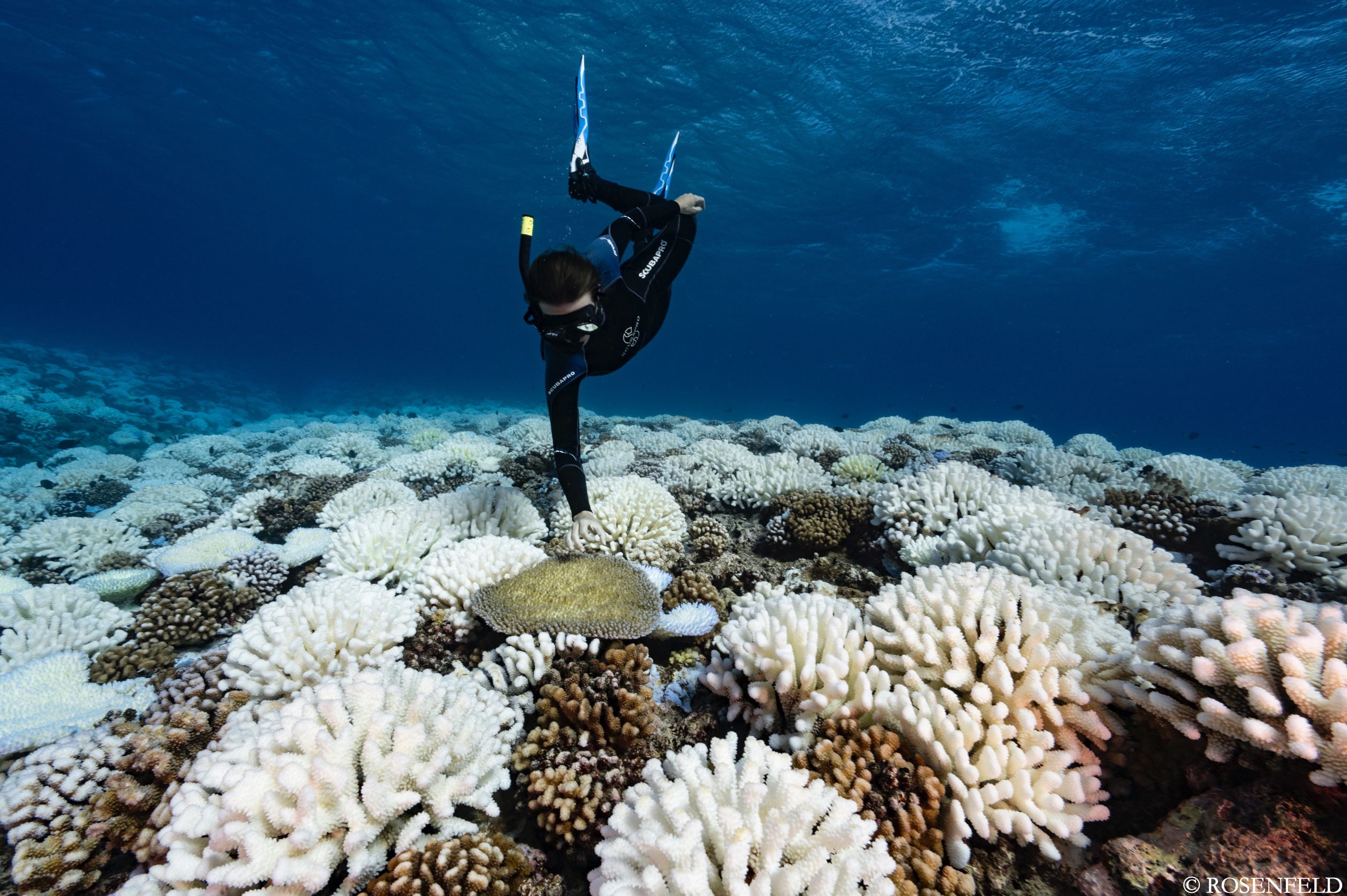
Coral Bleaching
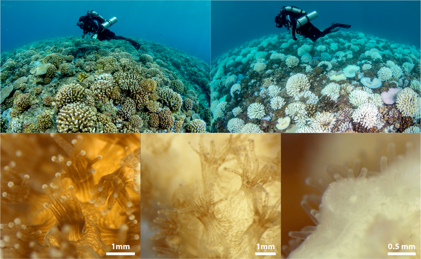
Coral Bleaching
Longterm Monitoring Data
Collected by CRIOBE since 2005
Point intercept transects
3 transects per site
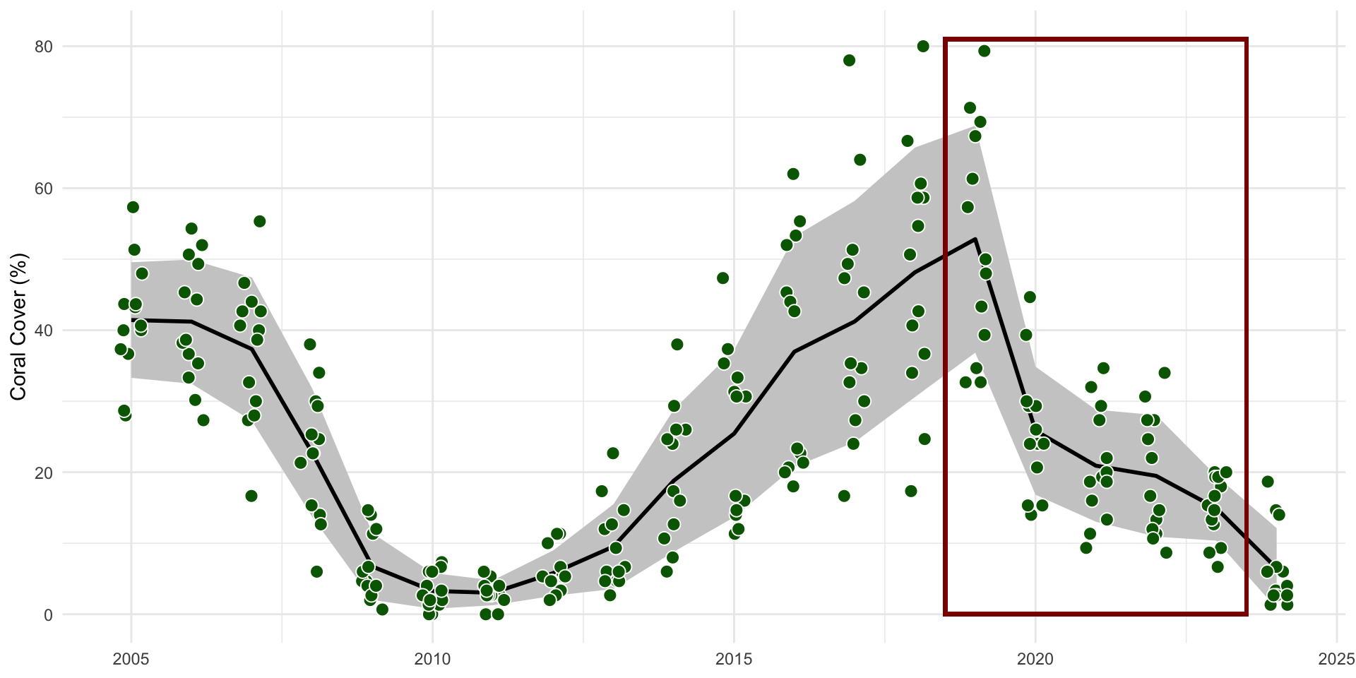
Longterm Monitoring Data
Task 2.2
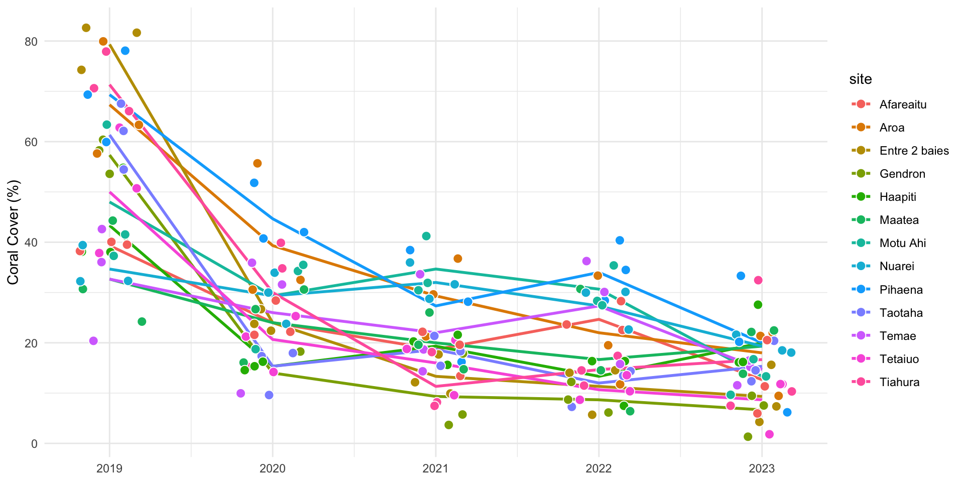
Make a similar plot
- The points are the mean
percentvalues per site - The line is the mean of these mean values
- The shaded area in this mean ± the standard deviation (sd())
Bleaching event 2019
Bleaching event 2019
Bleaching event 2019
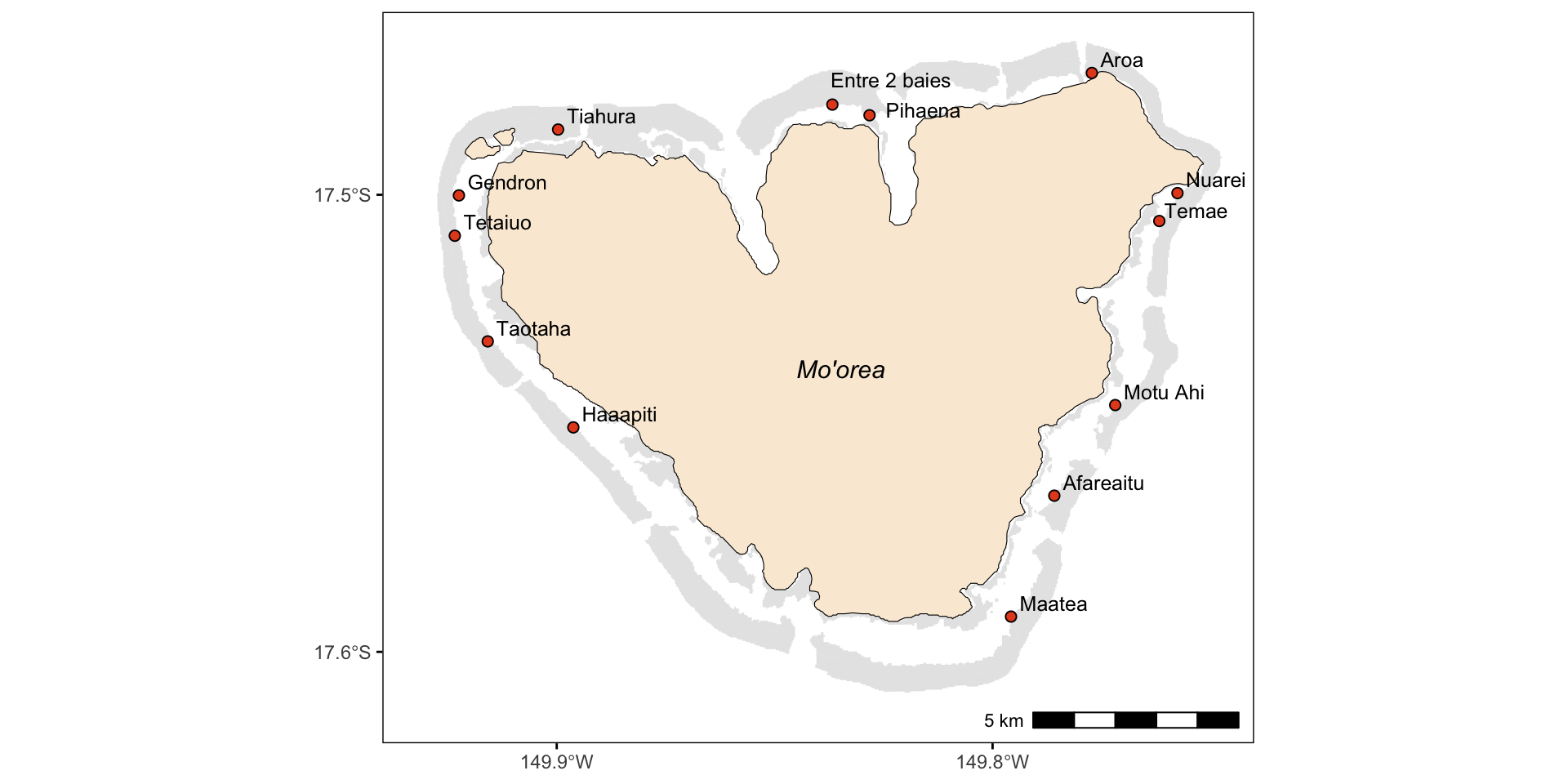
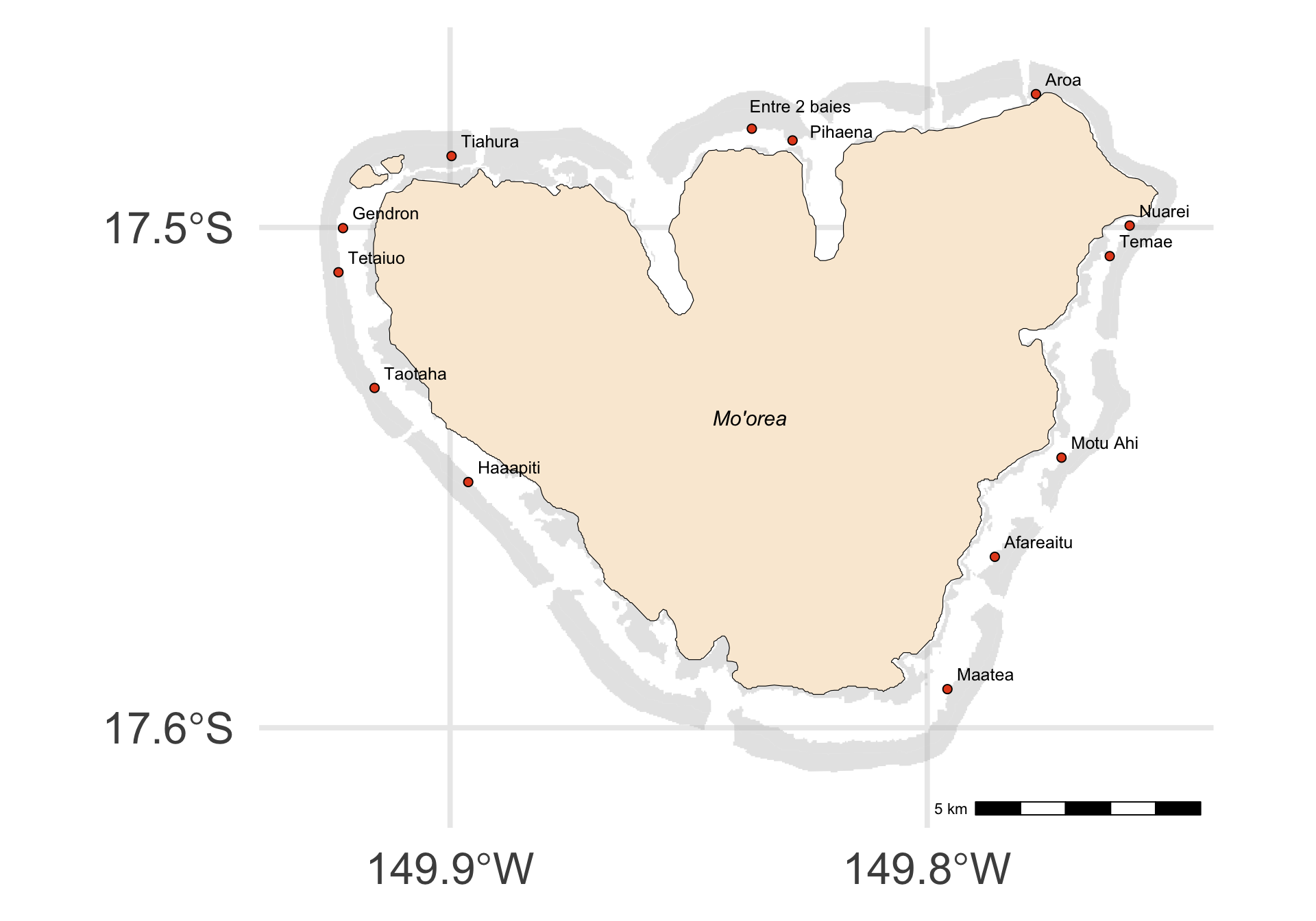
Bleaching event 2019 - Sites
Bleaching event 2019
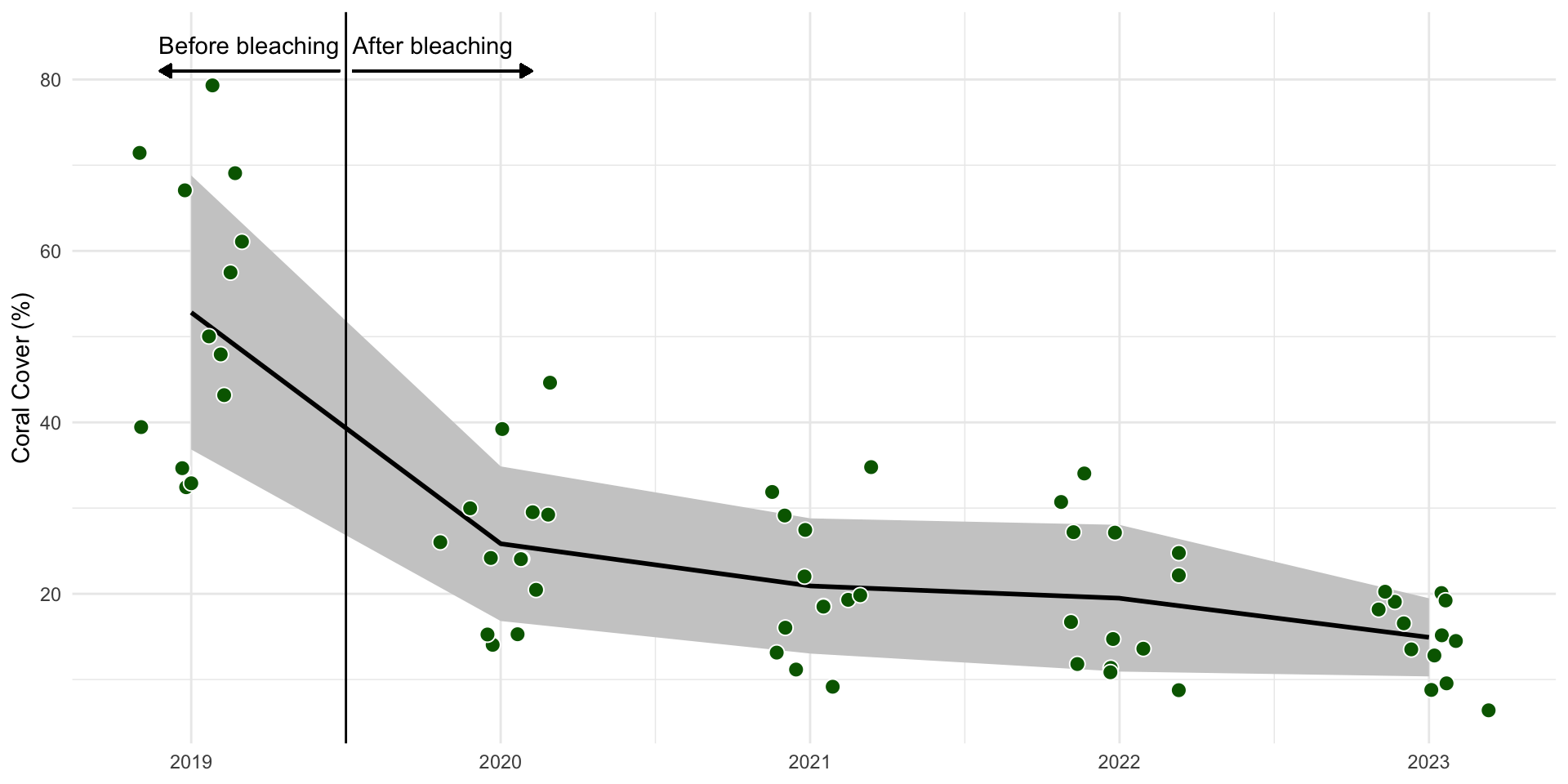
Task 2.3
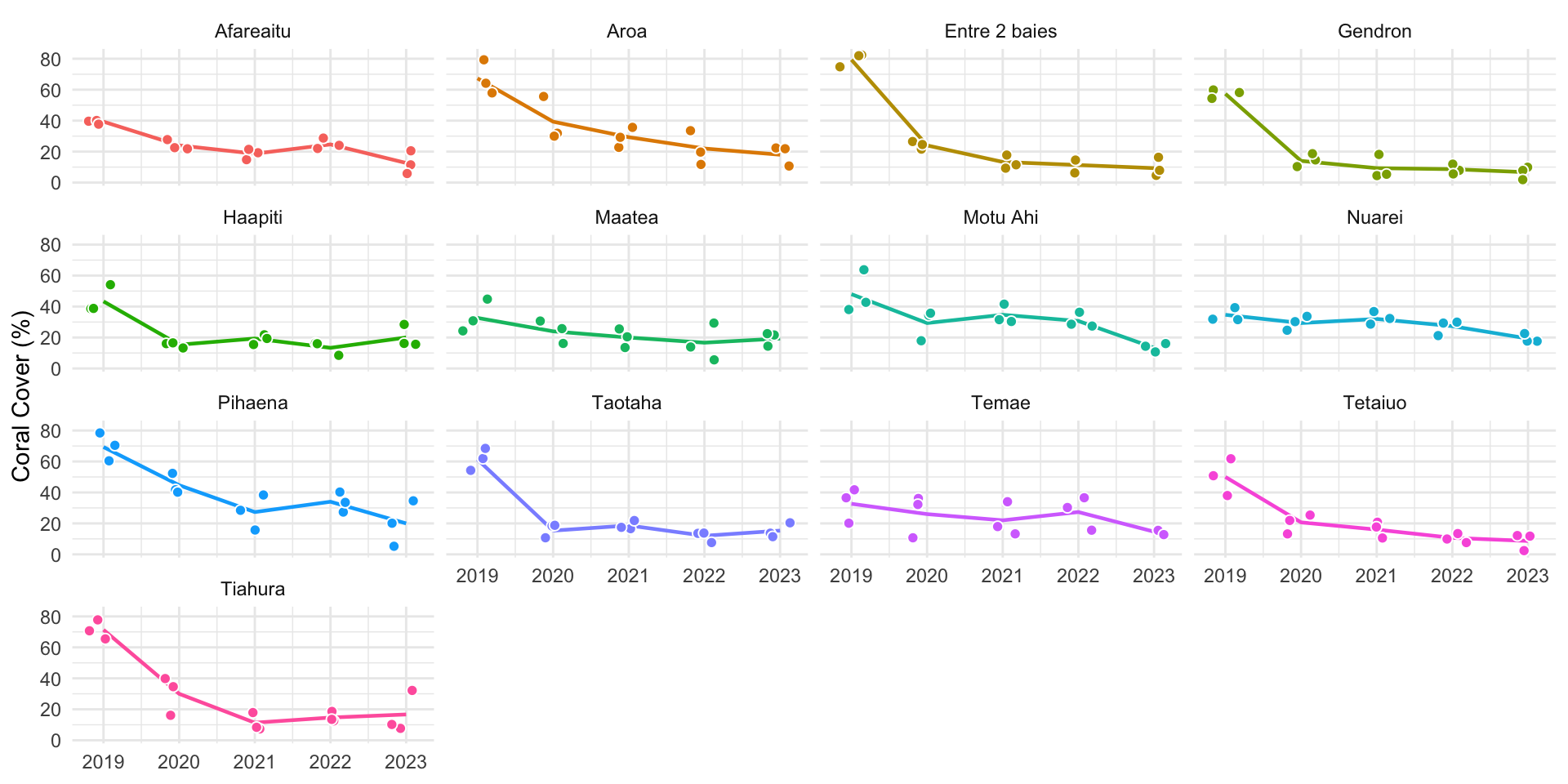
- Focus on data from 2019 until 2023
- Explore differences between sites
- How can you include the additional information?
- Lines on top of each other to show variability
- Different panels for each site to see what is happening where
- Other ideas?
Bleaching event 2019
Bleaching event 2019
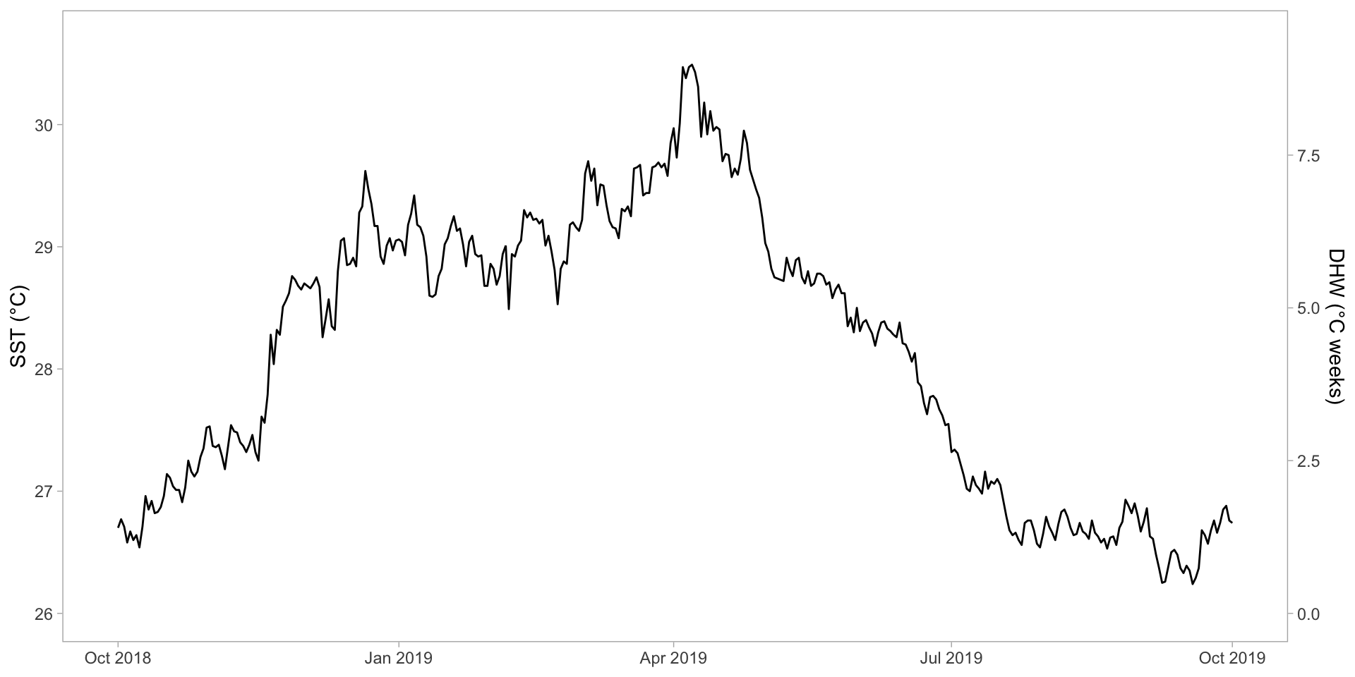
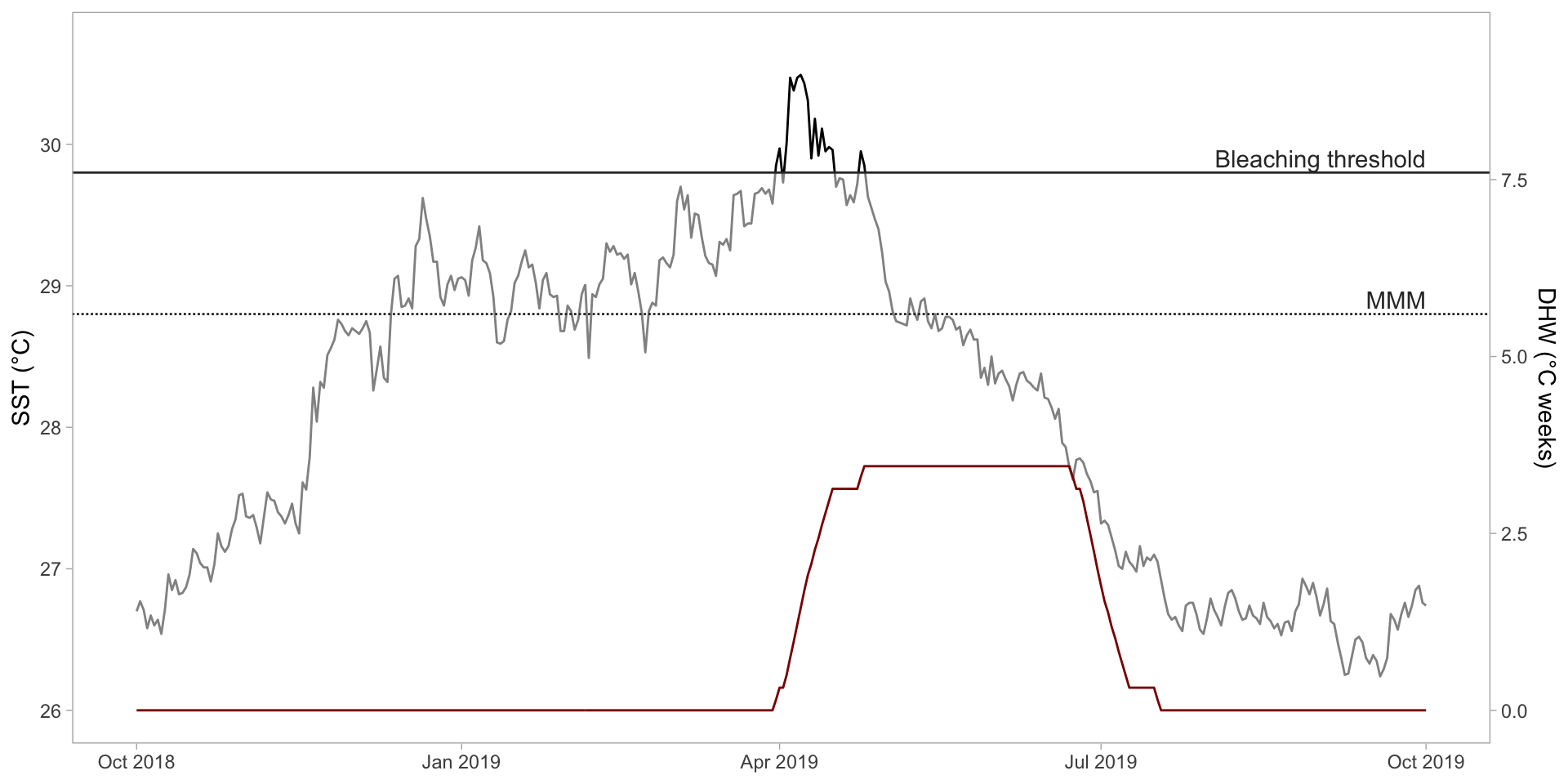
Degree Heating Weeks
- Measure for accumulated heat stress
- Satellite derived data
- Based on Sea Surface Temperature (SST)

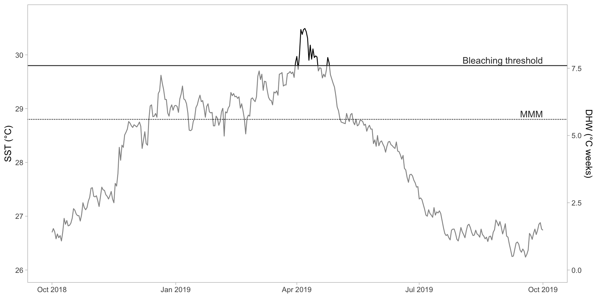
Calculation
Calculate difference between SST and bleaching threshold: long-term mean (MMM) + 1°C
Sum up all differences > 0 for the last 12 weeks (84 days)
Divide by 7 (=> unit is °C weeks)
Continue with next day
\[ \textrm{DHW} = \frac{1}{7}\sum_{i}^{84} BT\textrm{, where }BT \geq 1 \]
Degree Heating Weeks
Degree Heating Weeks
Degree Heating Weeks
Degree Heating Weeks
Degree Heating Weeks
Bleaching 2019
Strongest bleaching event in 30 years
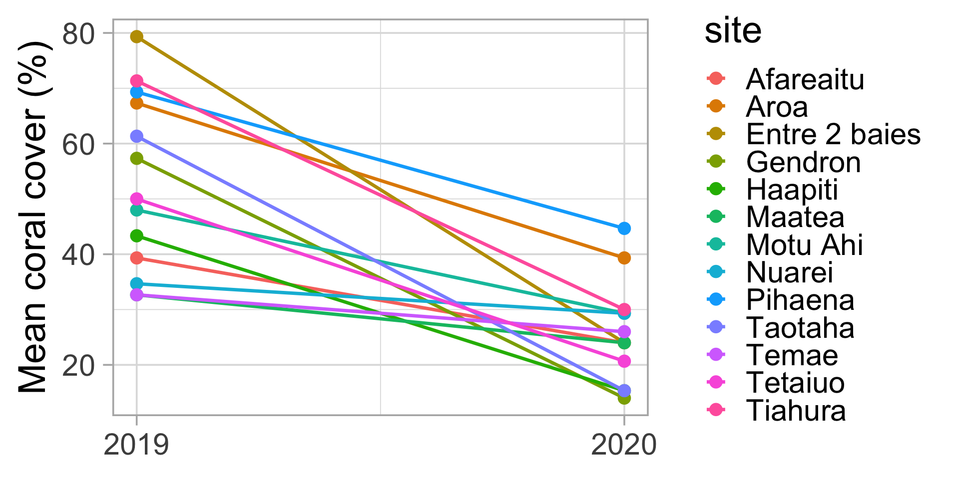
1. Change in cover
Aim
Calculate the change in coral cover in 2019 (before bleaching) and 2020 (after bleaching)
Considerations
The transect were not done at exactly the same spot => Transect 1 in 2020 not exactly at same spot as in 2019
Consequence
Calculate the mean cover per site and year before calculating the difference
![]()
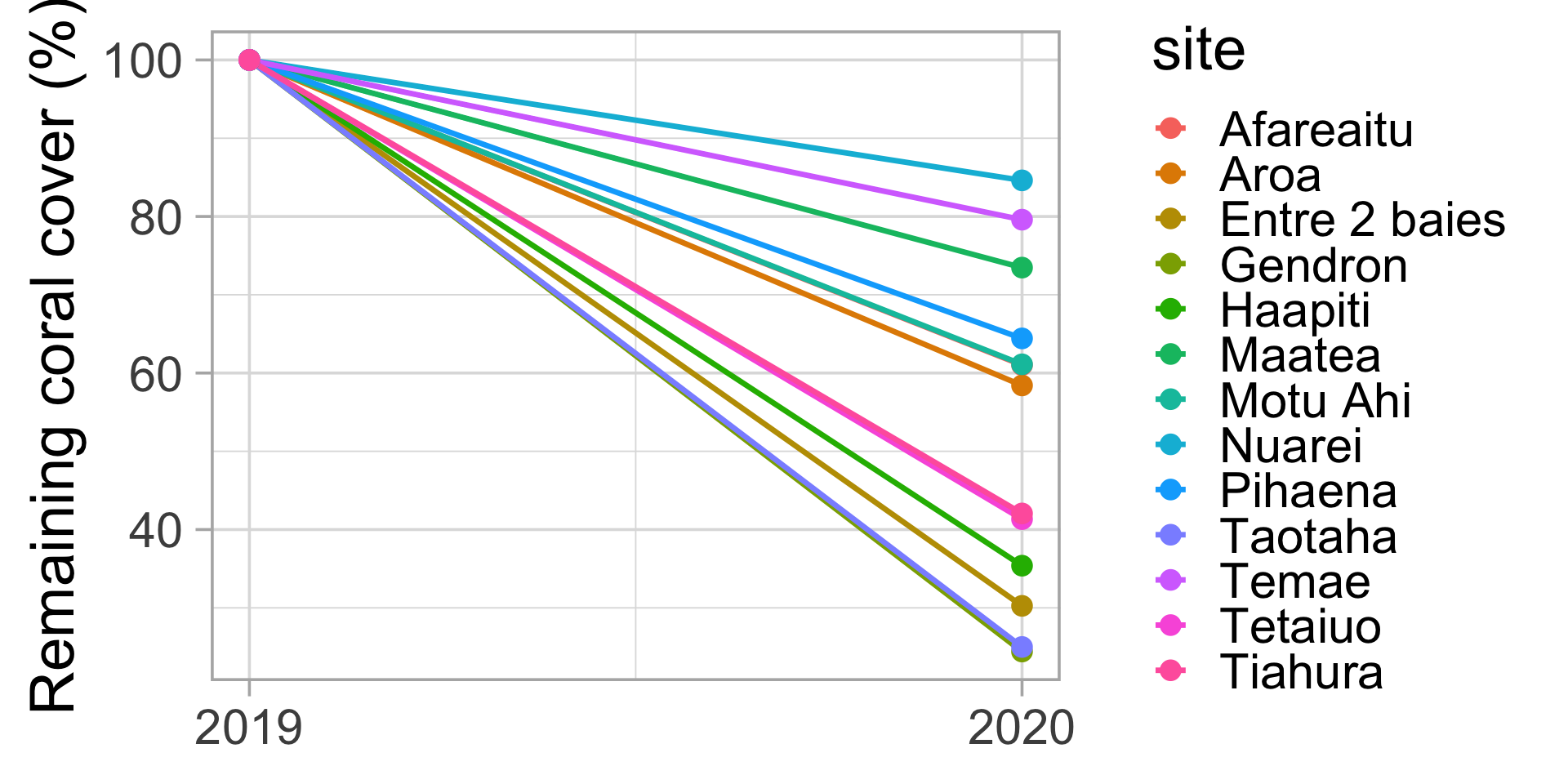
1. Change in cover
Aim
Calculate the change in coral cover in 2019 (before bleaching) and 2020 (after bleaching)
Considerations
The coral cover in 2019 differed between the sites, leading to different “start values”. This affects how much the cover can be reduced.
Consequence
Calculate the relative change in cover
dat_change_coral_cover <- dat_coral_cover %>%
filter(year >= 2019, year <= 2020) %>%
group_by(site, year) %>%
summarise(percent = mean(percent)) %>%
pivot_wider(names_from = year,
values_from = percent) %>%
# calculate relative change
mutate(rel_change = 100*(`2019` - `2020`)/`2019`) %>%
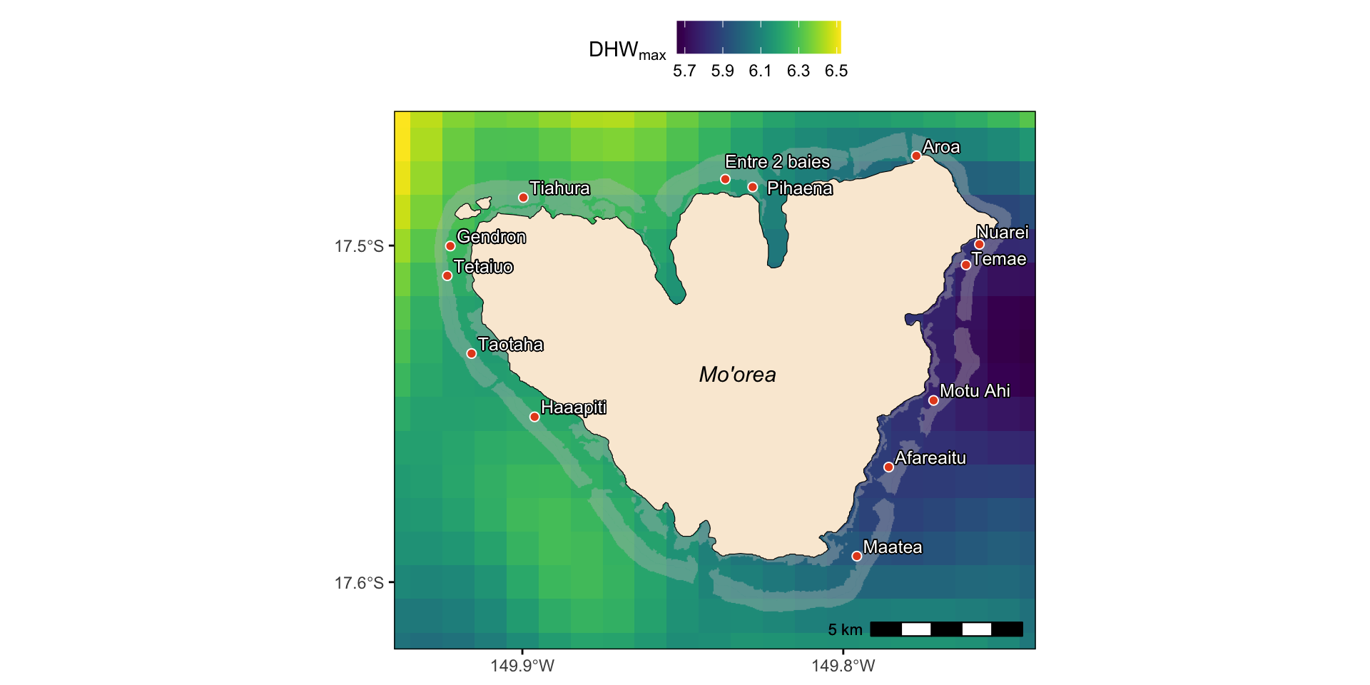
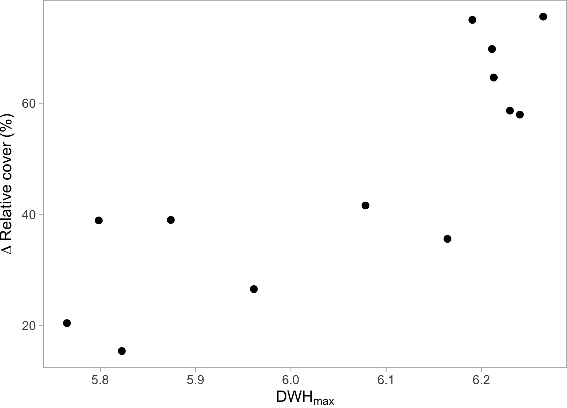
select(-`2020`, -`2019`)2. DWHmax

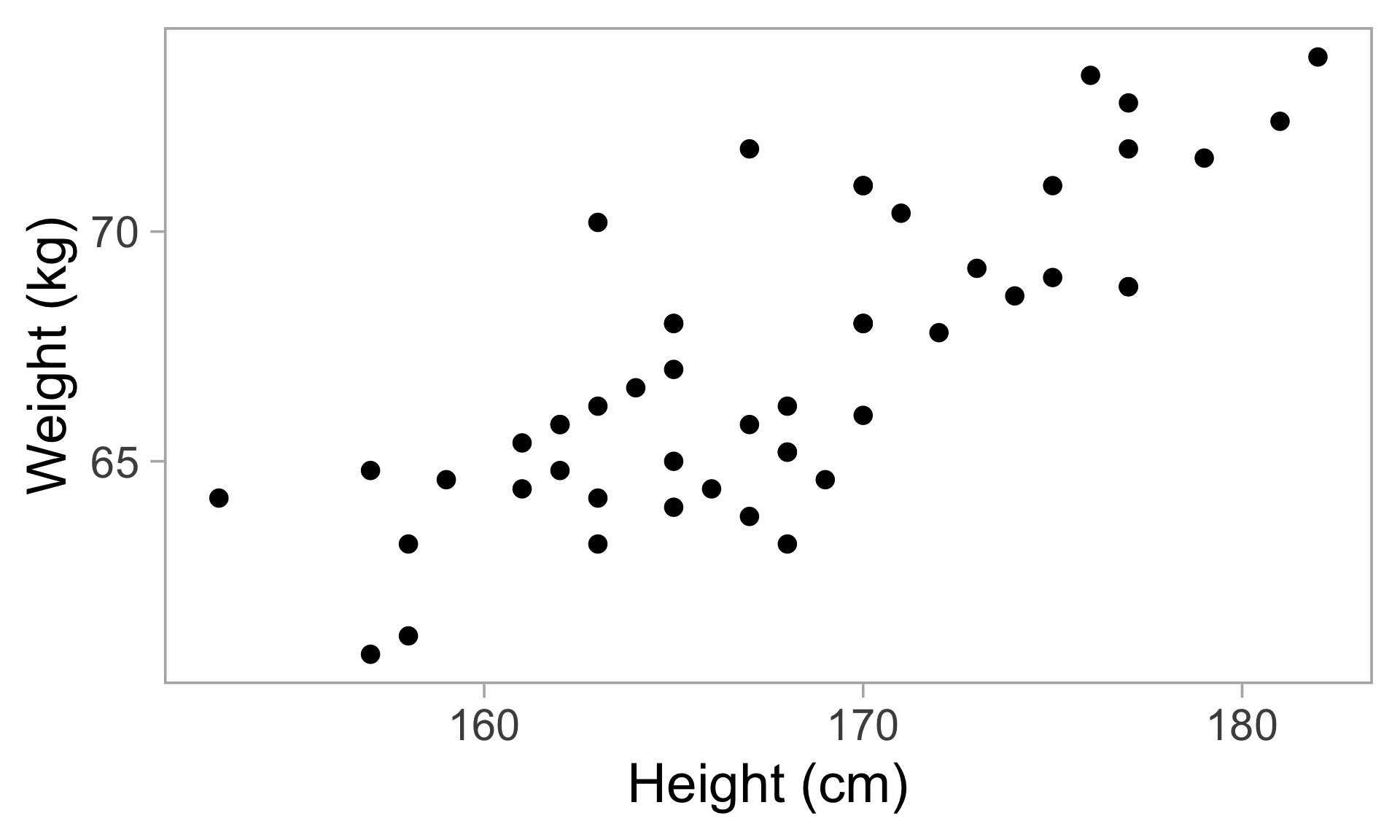
3. Regression
Type of linear model
Tries to explain how one variable (e.g. height) influences another (e.g. weight)
Can be used to
predict e.g. weight only with height
assess importance (significant or not)
3. Regression
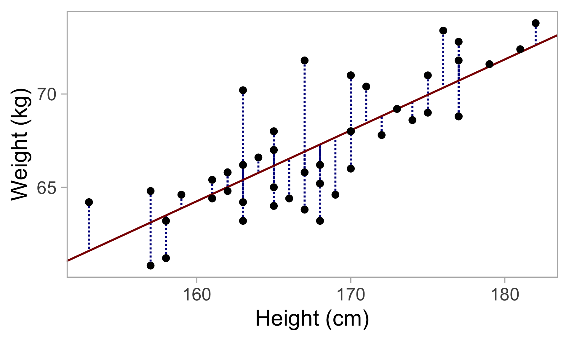
Finds the best fitting line through a point cloud
\[ y_i = a + b x_i + \epsilon_i \]
\(a\) is the y-intercept, \(b\) is the slope
\(y_i\) is the expected y value at \(x_i\)
The data does not fit perfectly to the line, each actual data point can vary by \(\epsilon\)

3. Regression
Example
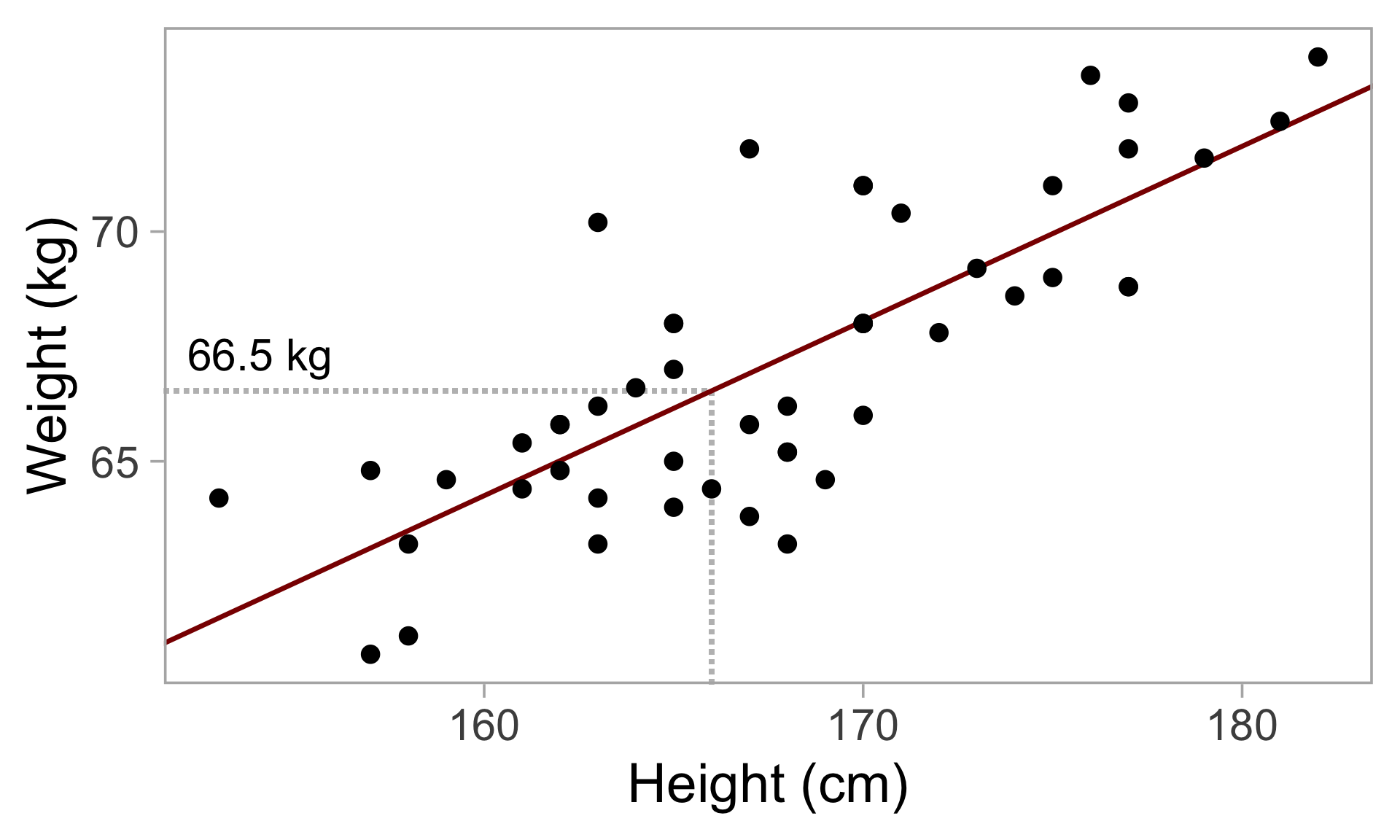
- Here, \(a\) = 3.41 and \(b\) = 0.38
What is the expected weight for a height of 166 cm?
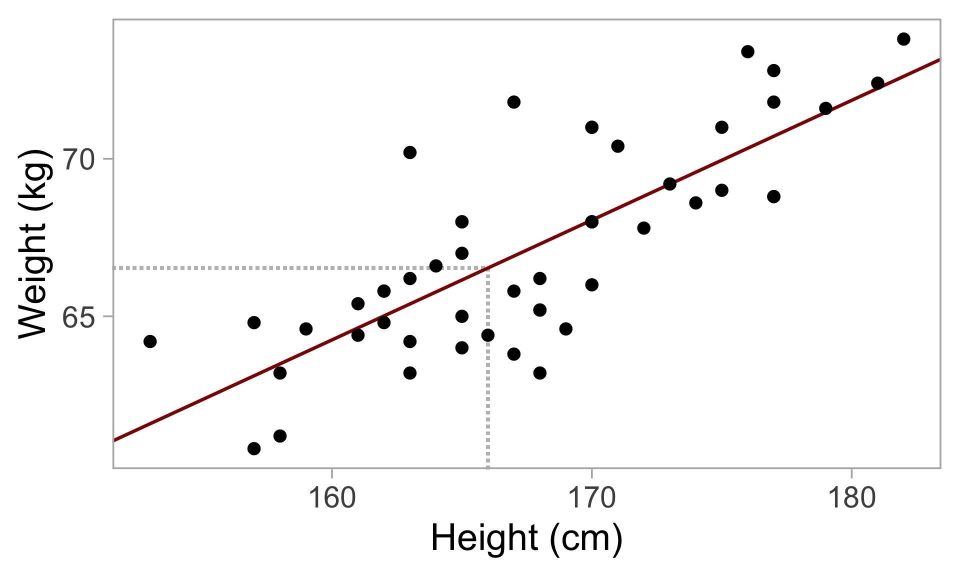
3. Regression
Example
Here, \(a\) = 3.41 and \(b\) = 0.38
Expected weight for a height of 166 cm is 66.5 kg
3. Regression
Example
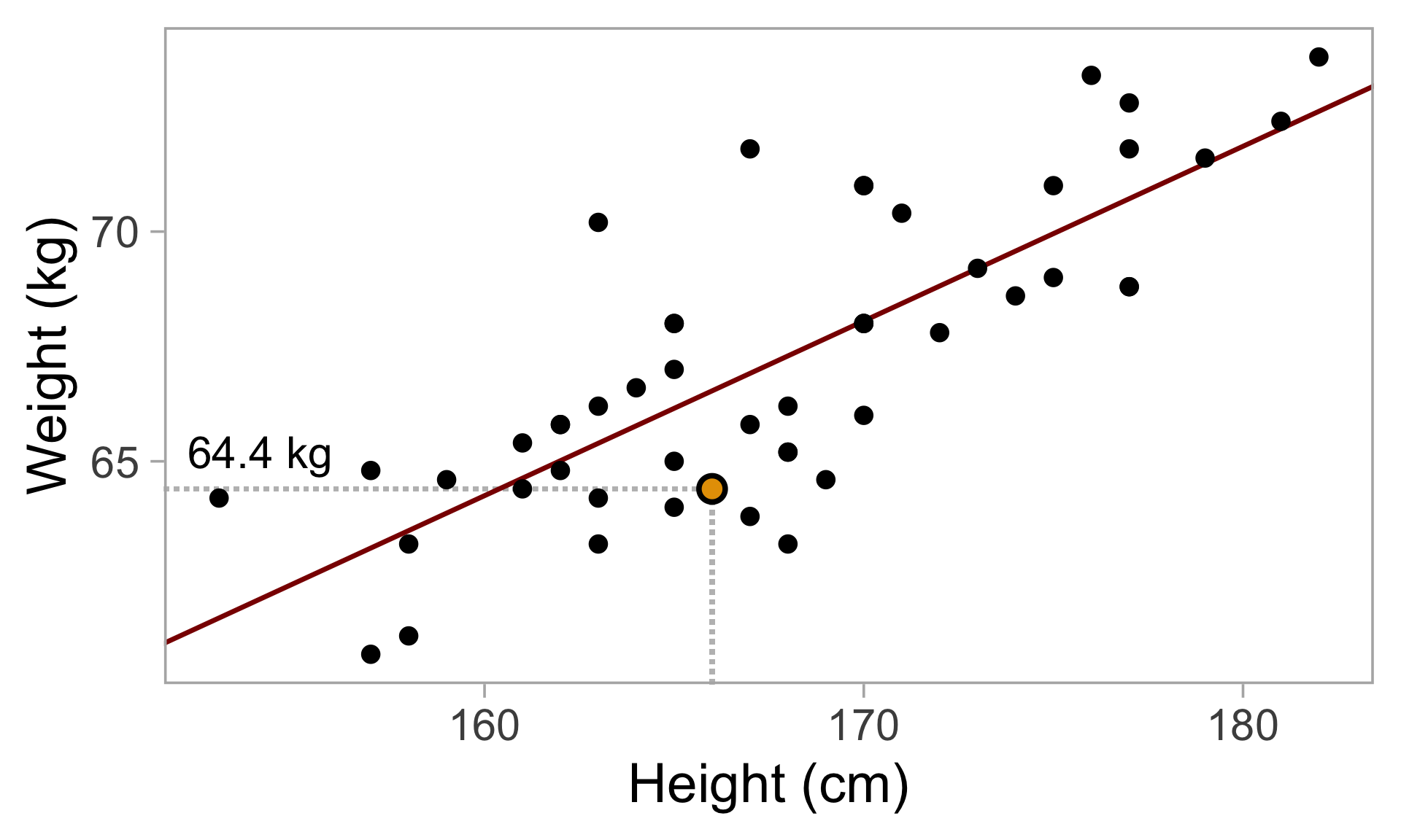
Here, \(a\) = 3.41 and \(b\) = 0.38
Expected weight for a height of 166 cm is 66.5 kg
In the actual data, the corresponding weight is 64.4 kg
3. Regression
Example
Here, \(a\) = 3.41 and \(b\) = 0.38
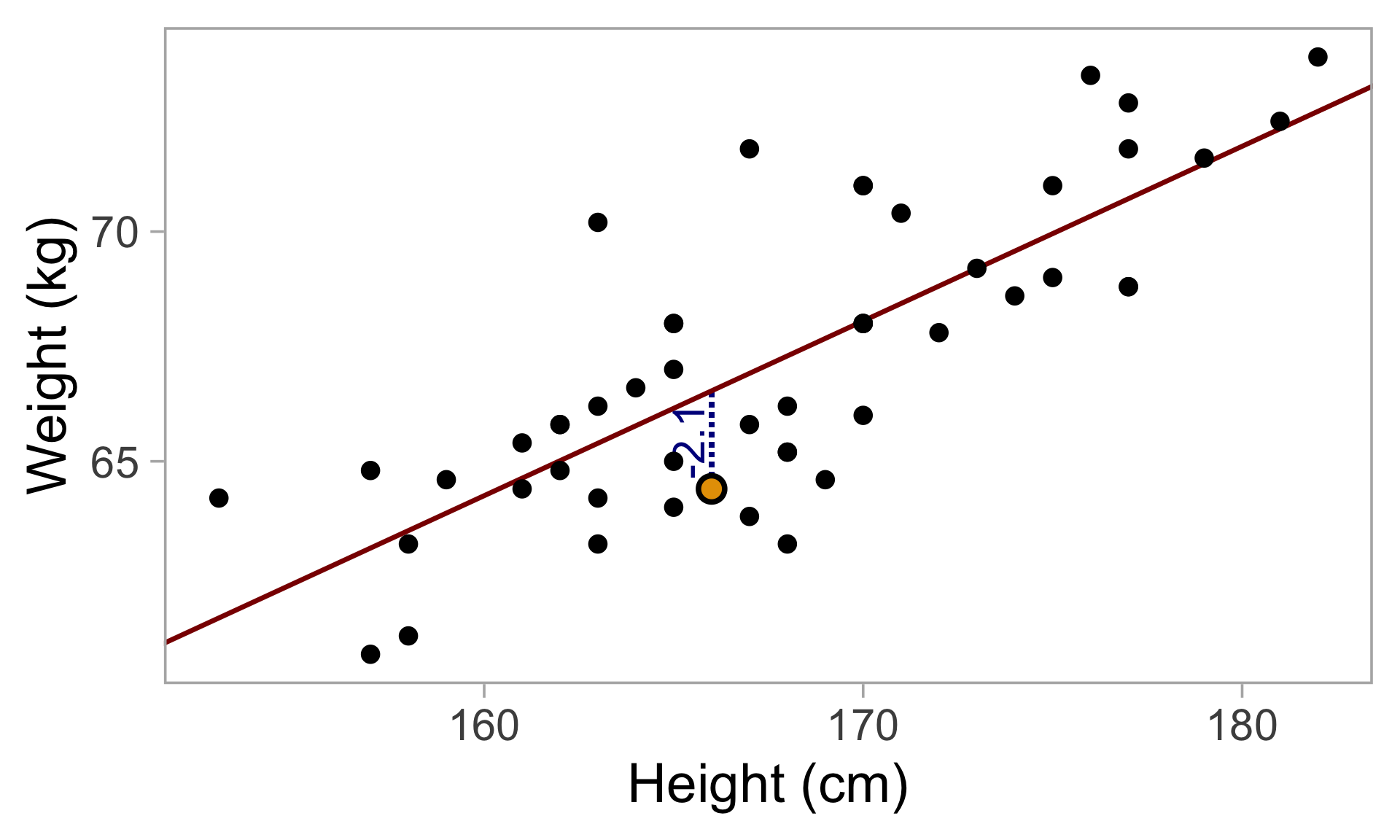
Expected weight for a height of 166 cm is 66.5 kg
In the actual data, the corresponding weight is 64.4 kg
At this point, the error \(\epsilon_{166~cm}\) is -2.1 kg
3. Regression
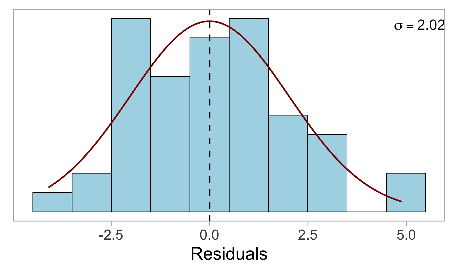
Residuals
These errors are called residuals
Over all the data points, the residuals are expected to follow a normal distribution with mean 0 (to allow positive and negative values) and standard deviation (\(\sigma\)):
\(\epsilon \sim normal(0, \sigma)\)
- The standard deviation (\(\sigma\)) is calculated by the linear model function

3. Regression
Residuals
3. Regression
Task 2.5
Back to the coral cover data set
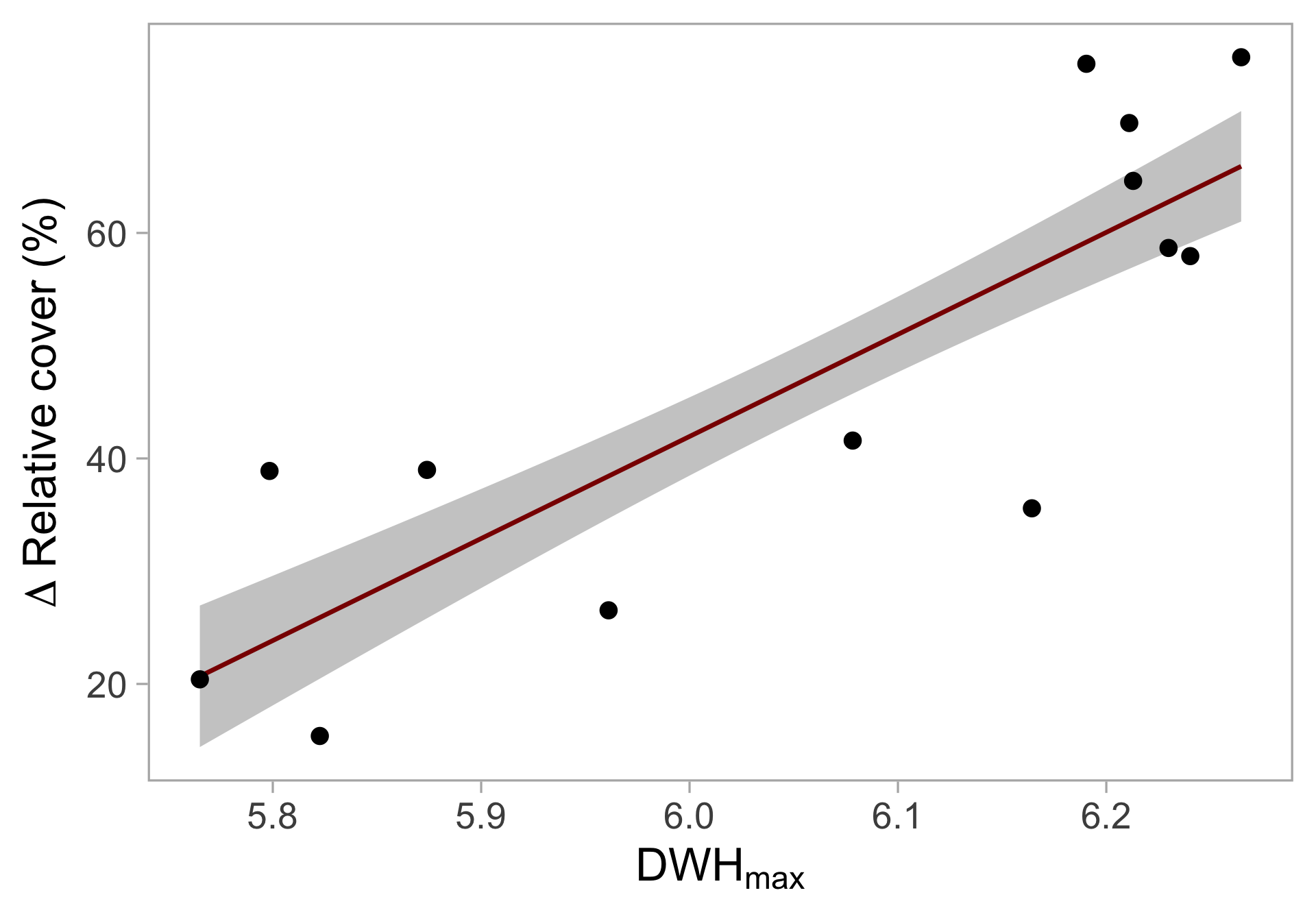
Analyse the impact of max_dhw on rel_change
Is this effect significant?
What is the expected change in coral cover per unit DHW?
4. Visualisation
Weight data set
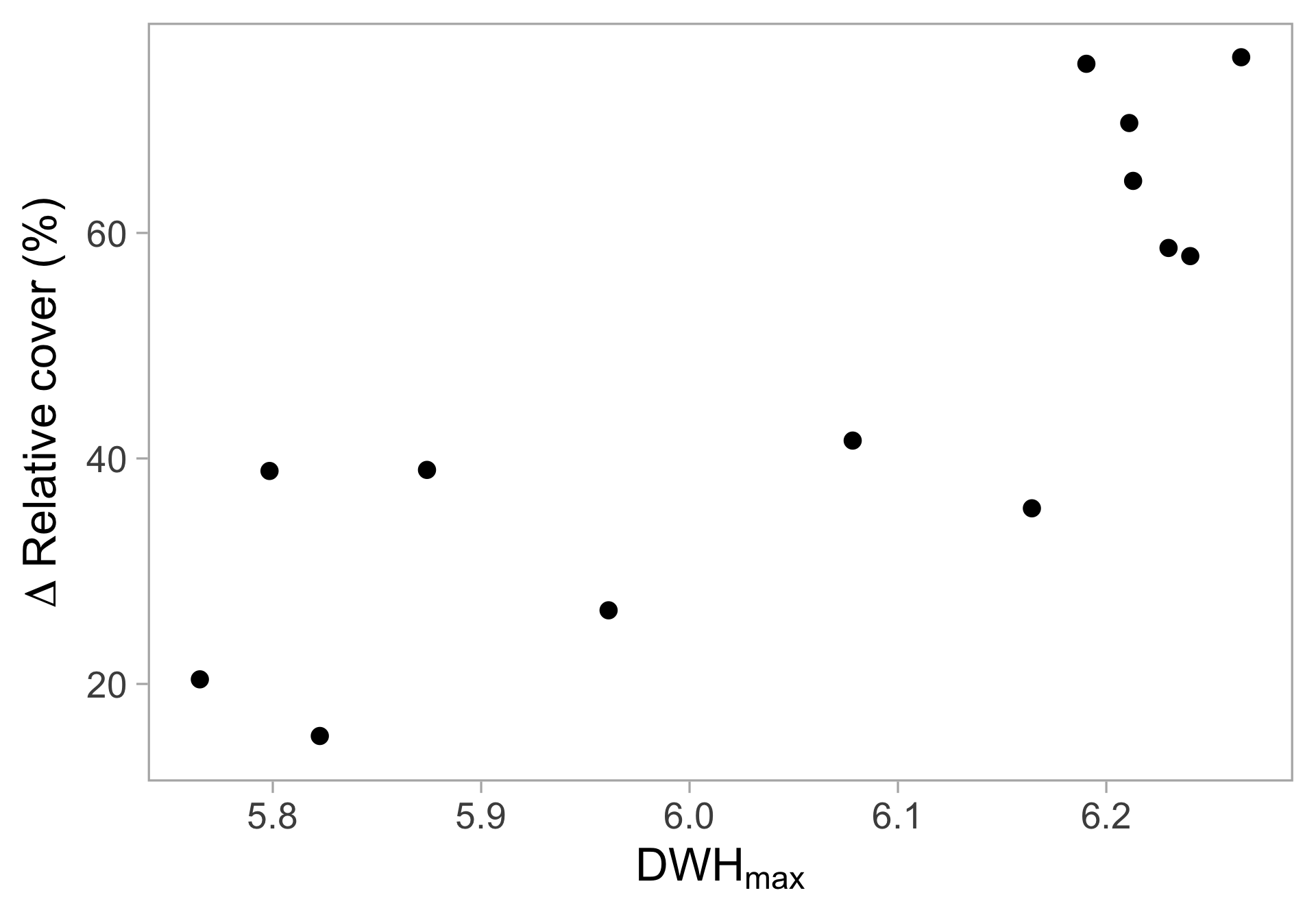
Layers
- Raw Data
4. Visualisation
Weight data set
Layers
- Raw Data
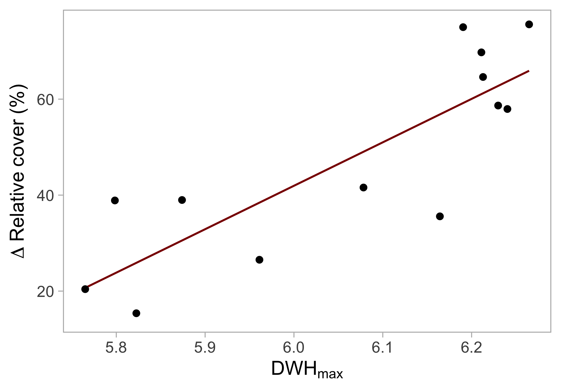
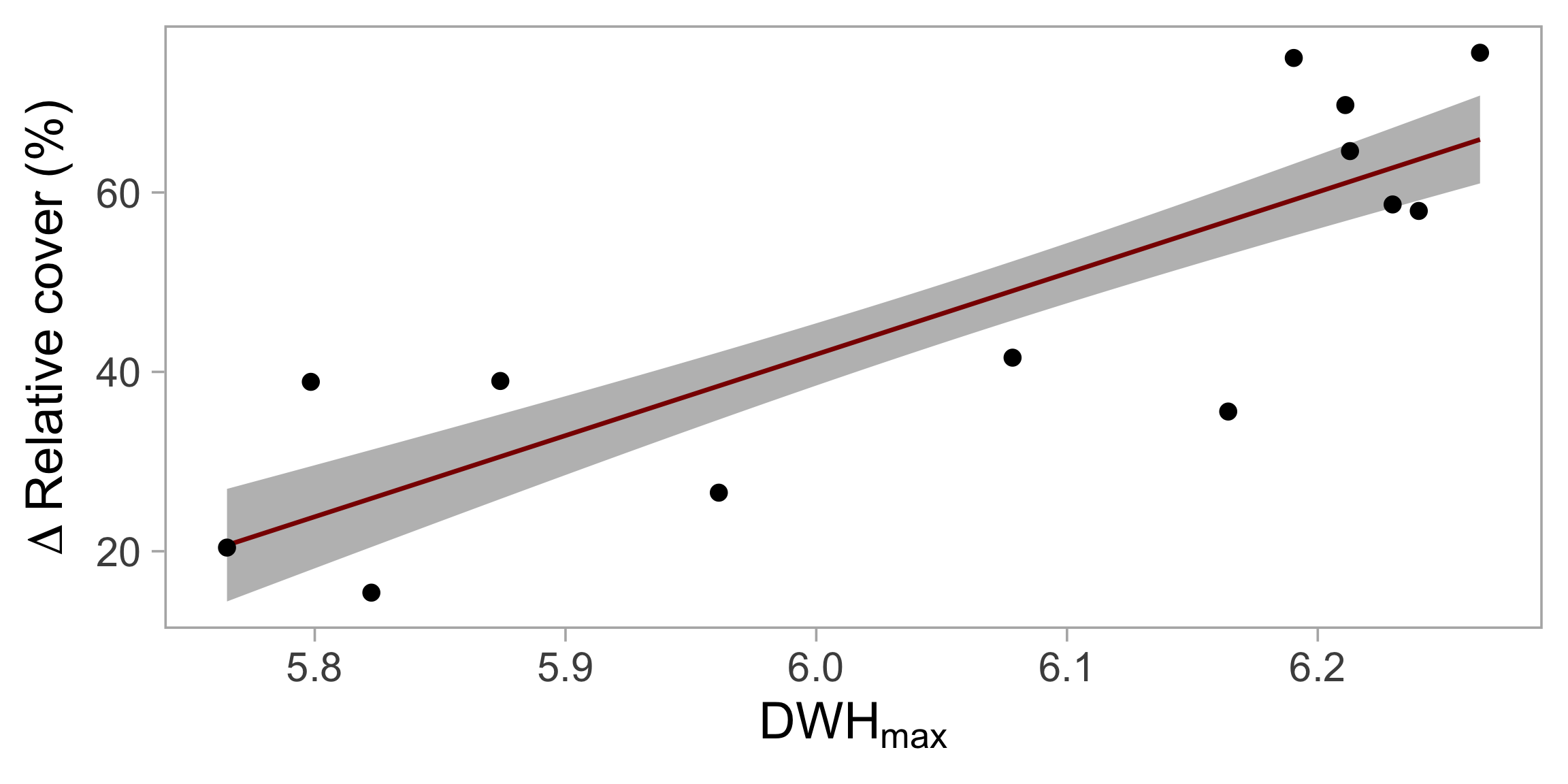
- Linear equation:
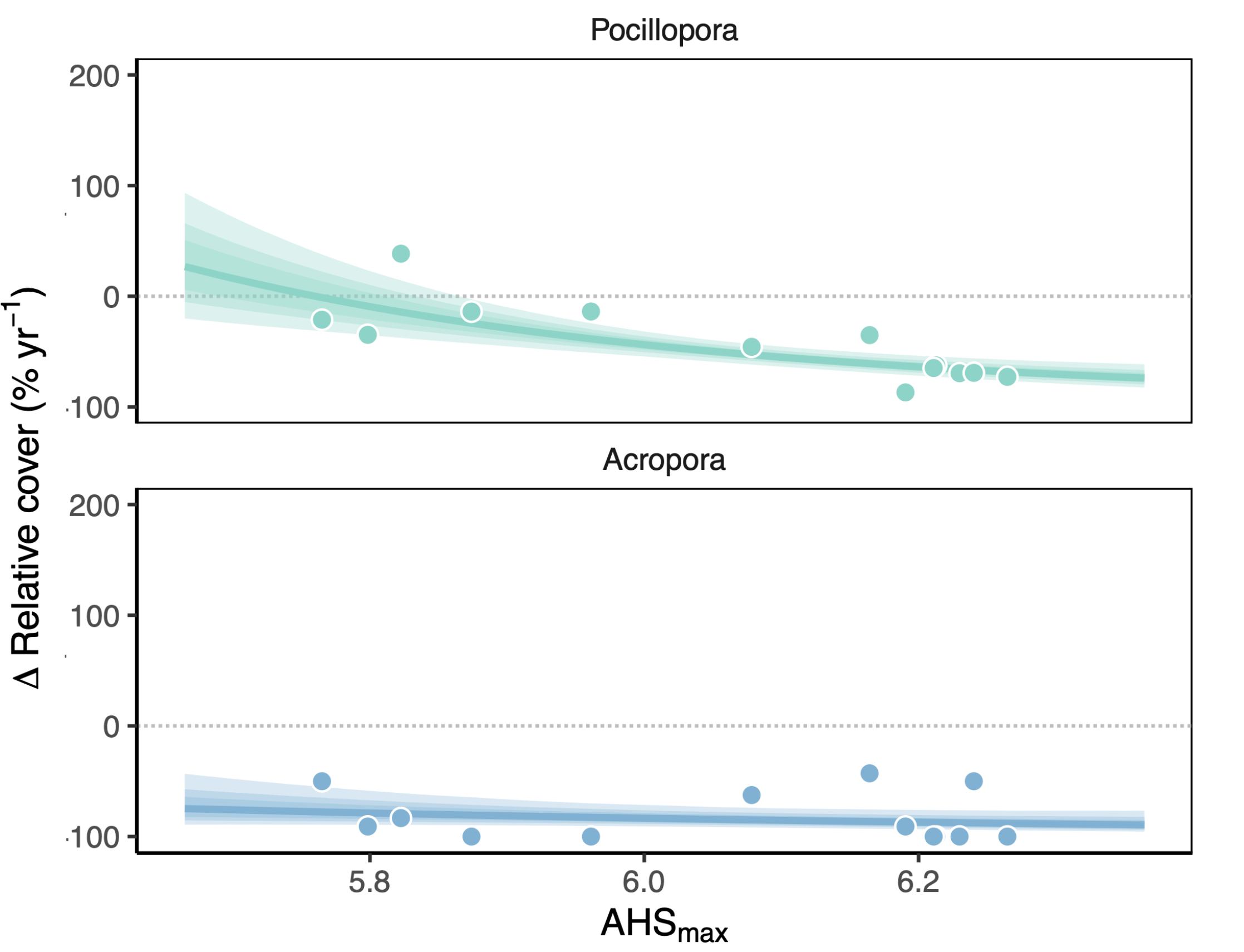
\(\Delta\) Relative cover = -501.2 + 90.5 * DHWmax
4. Visualisation
Weight data set
Layers
- Raw Data
- Linear equation:
\(\Delta\) Relative cover = -501.2 + 90.5 * DHWmax
- Standard error of predictions
4. Visualisation
Task 2.6
Plot the coral cover data and model in a similar way
Thermotolerance
Many studies show that the thermotlerance differs between genera and species!
Thermotolerance