Environmental Risk
Part 1
RStudio
![]()
Programming language
Special language for statistical analyses and visualizations

Interface to R
Provides a layout and functions that make it easier and more efficient to use R
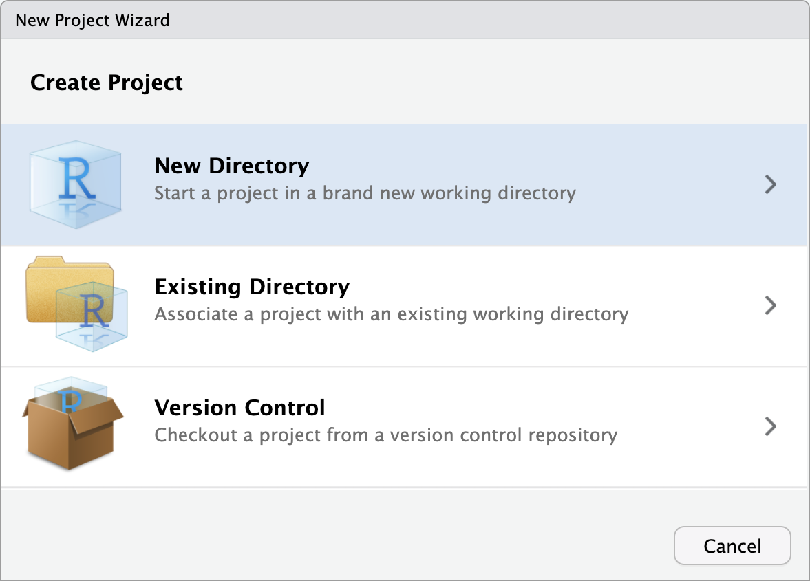
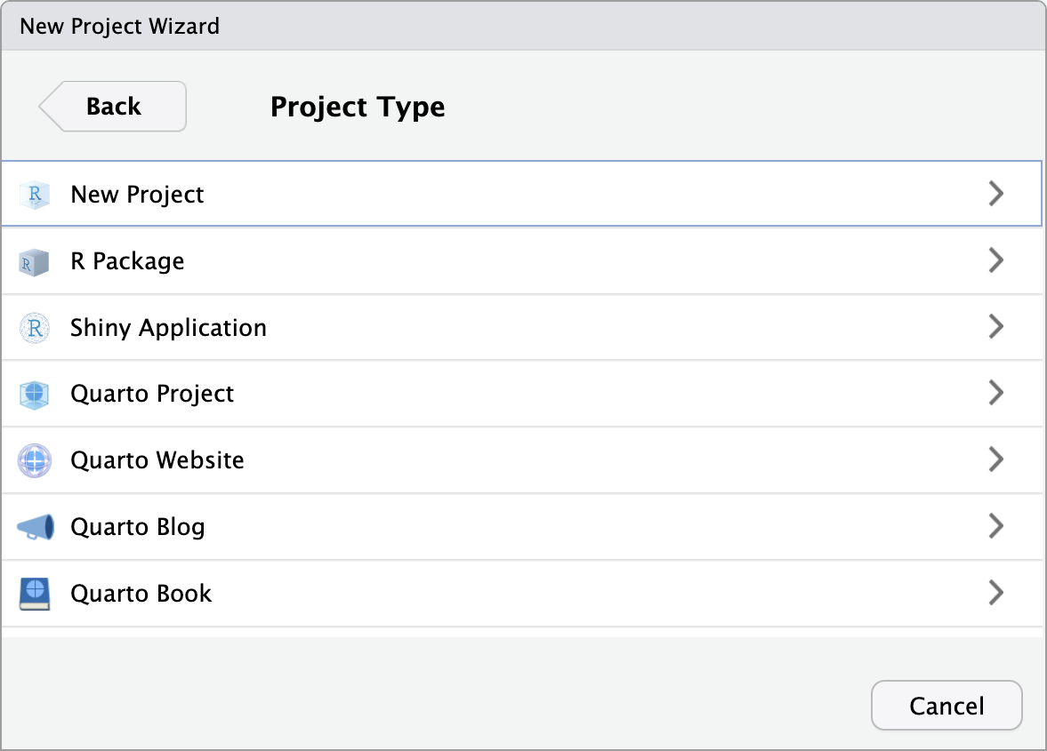
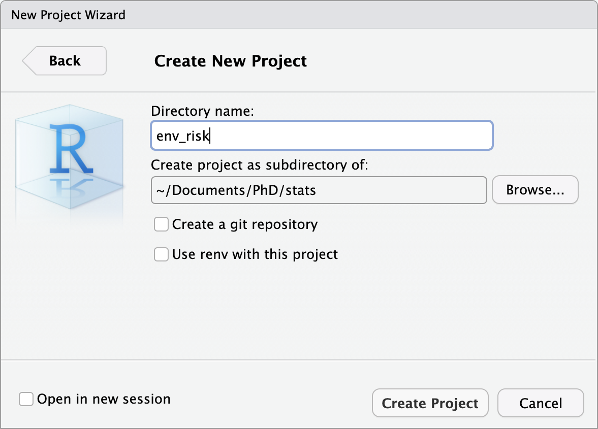
Create Project
→
Folder Structure
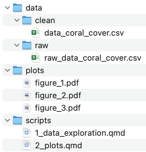
data: All data used for you analysis. Keep in it a folder with all raw data that you do not touch
scripts: All scrips for your analysis. You can keep it organised with numbers, e.g.
1_data_exploration.qmd2_plots.qmd
plots: Plots generated during your analysis
Use Quarto Documents
→ →
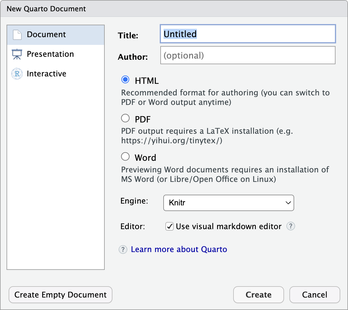
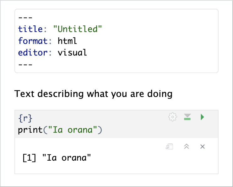
Use Quarto Documents
Insert R code with  or on Mac Option-Command-IOption-Command-I or Windows Control-Alt-OControl-Alt-O
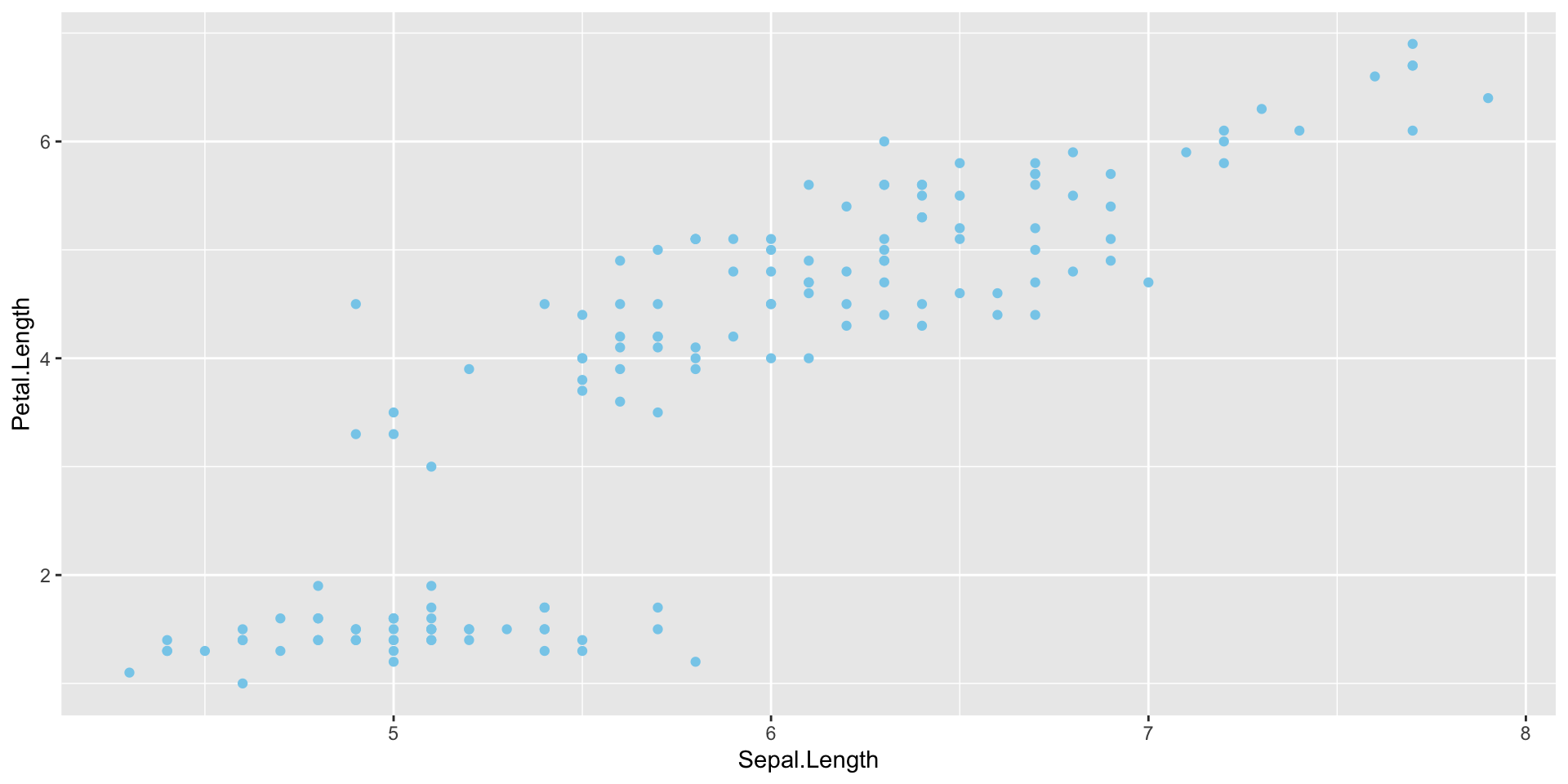
tidyverse package
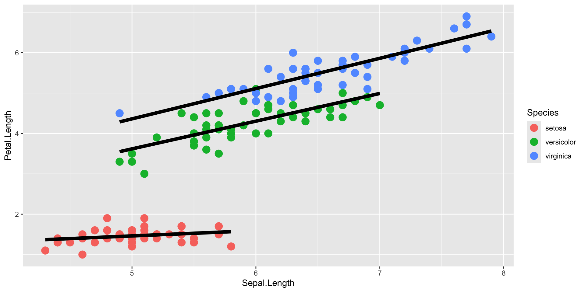
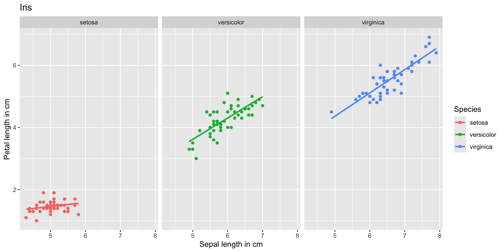
Introduction to ggplot2 package
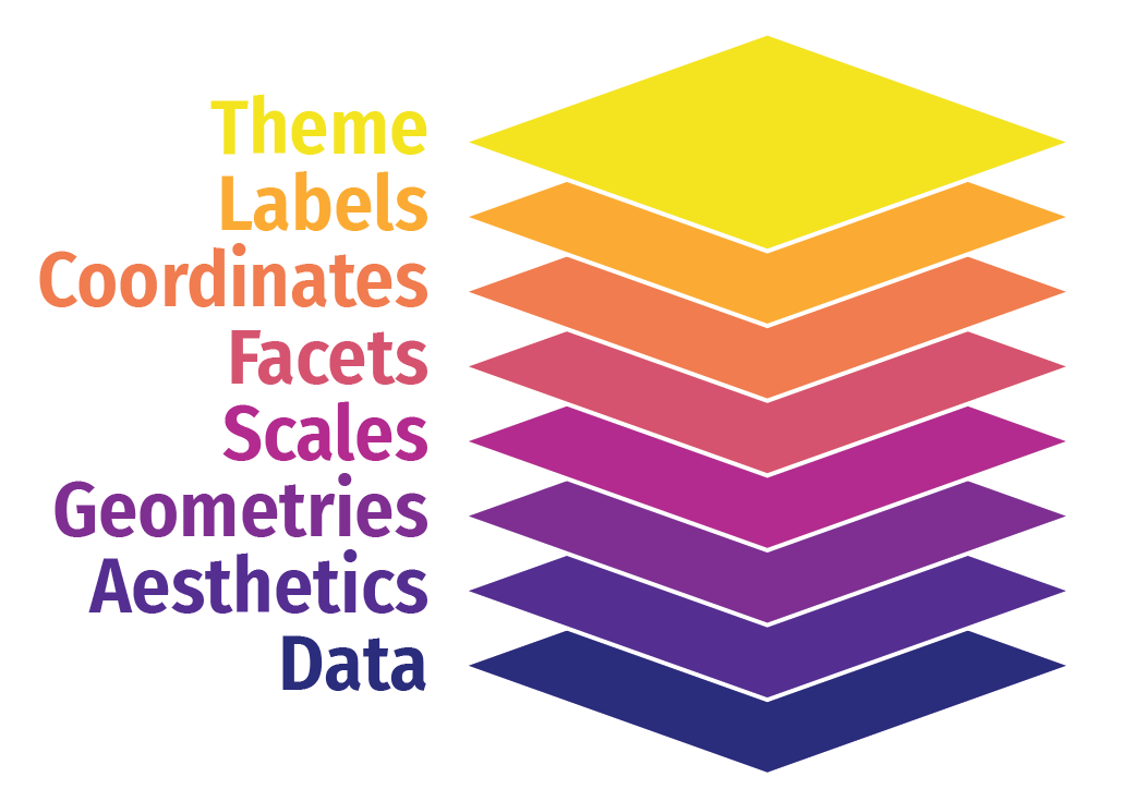
Workflow
- Data
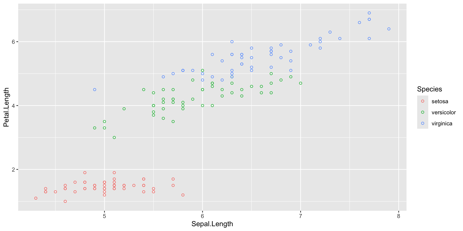
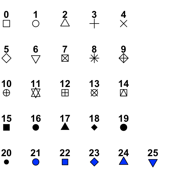
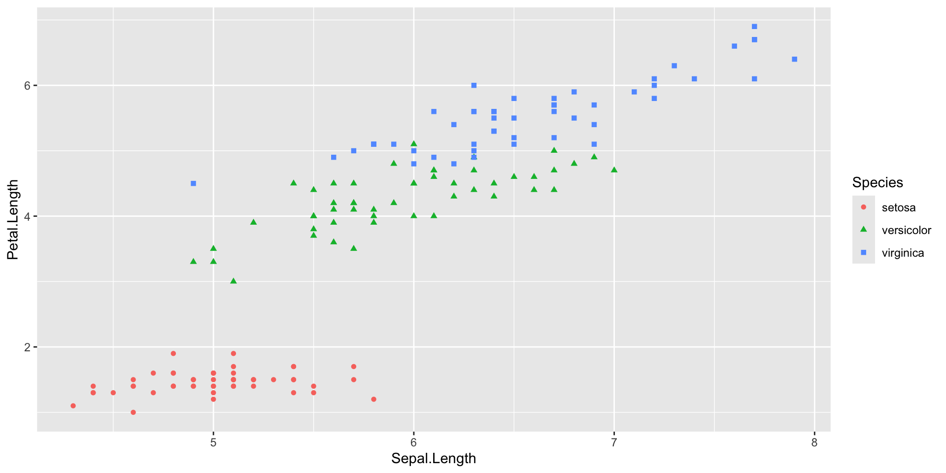
- Mapping: x and y coordinates, colors, point shapes, etc (
aes()) - Layer type: points, lines, etc (
geom_...()) - Additional formatting, as subplots, specific colors, labels, plot title, etc.
- Themes for text size, style, etc.
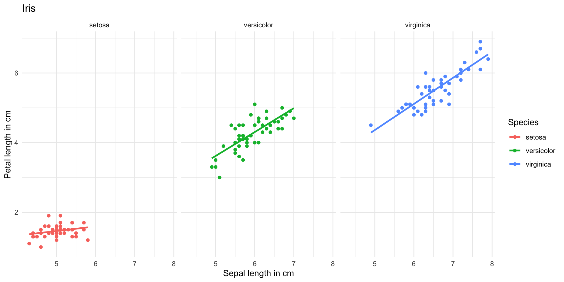
Introduction to ggplot2 package
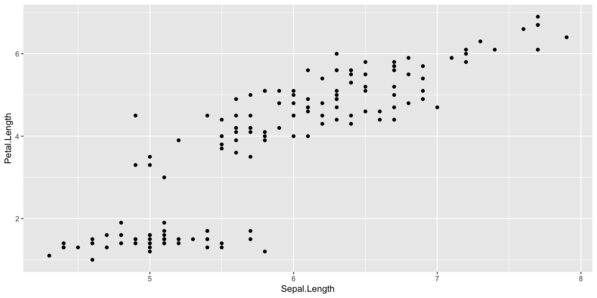
Introduction to ggplot2 package
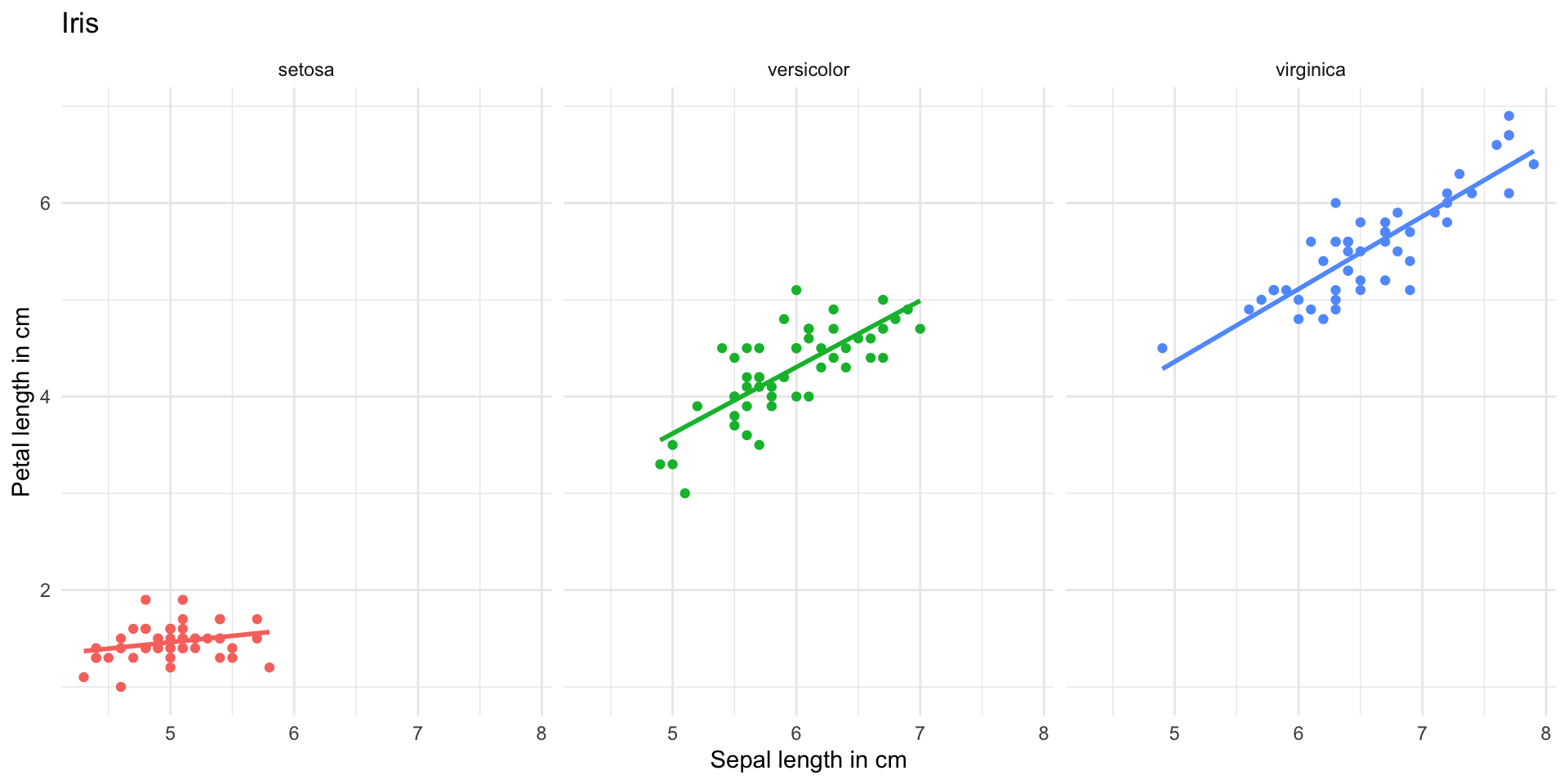
Introduction to ggplot2 package
Introduction to ggplot2 package
Introduction to ggplot2 package
Introduction to ggplot2 package

Introduction to ggplot2 package
Introduction to ggplot2 package
Introduction to ggplot2 package
Introduction to ggplot2 package
Introduction to ggplot2 package
Introduction to ggplot2 package
Introduction to ggplot2 package
Introduction to ggplot2 package
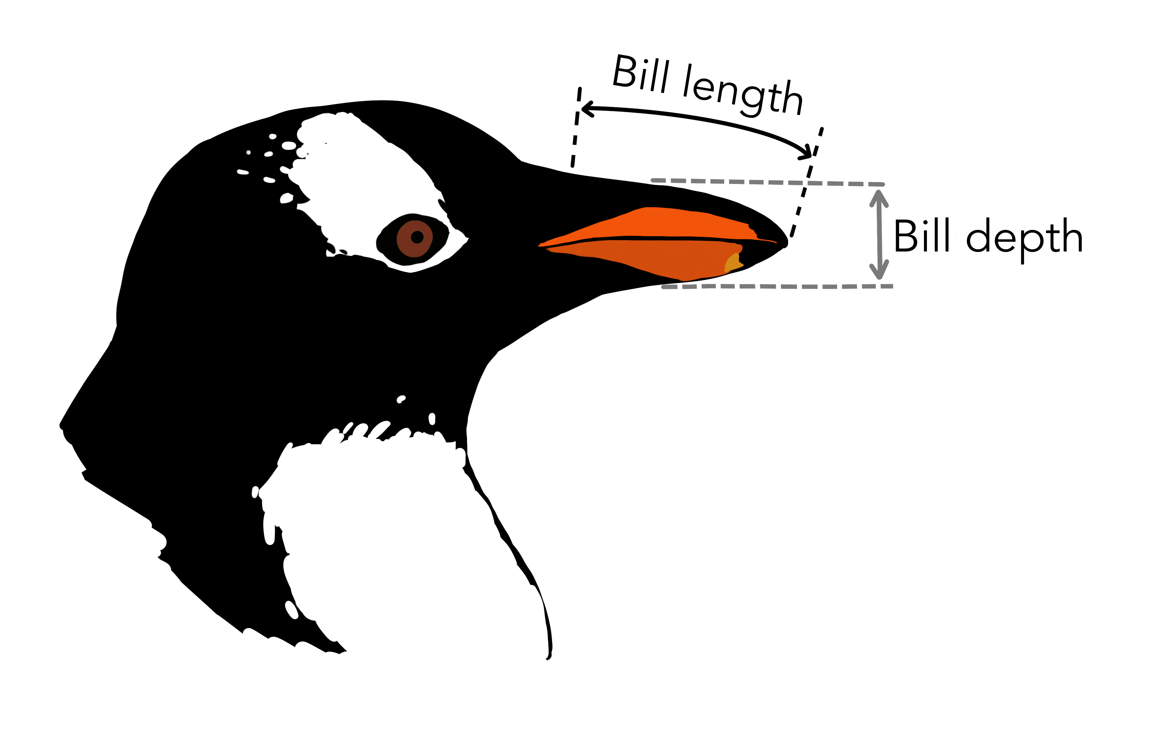
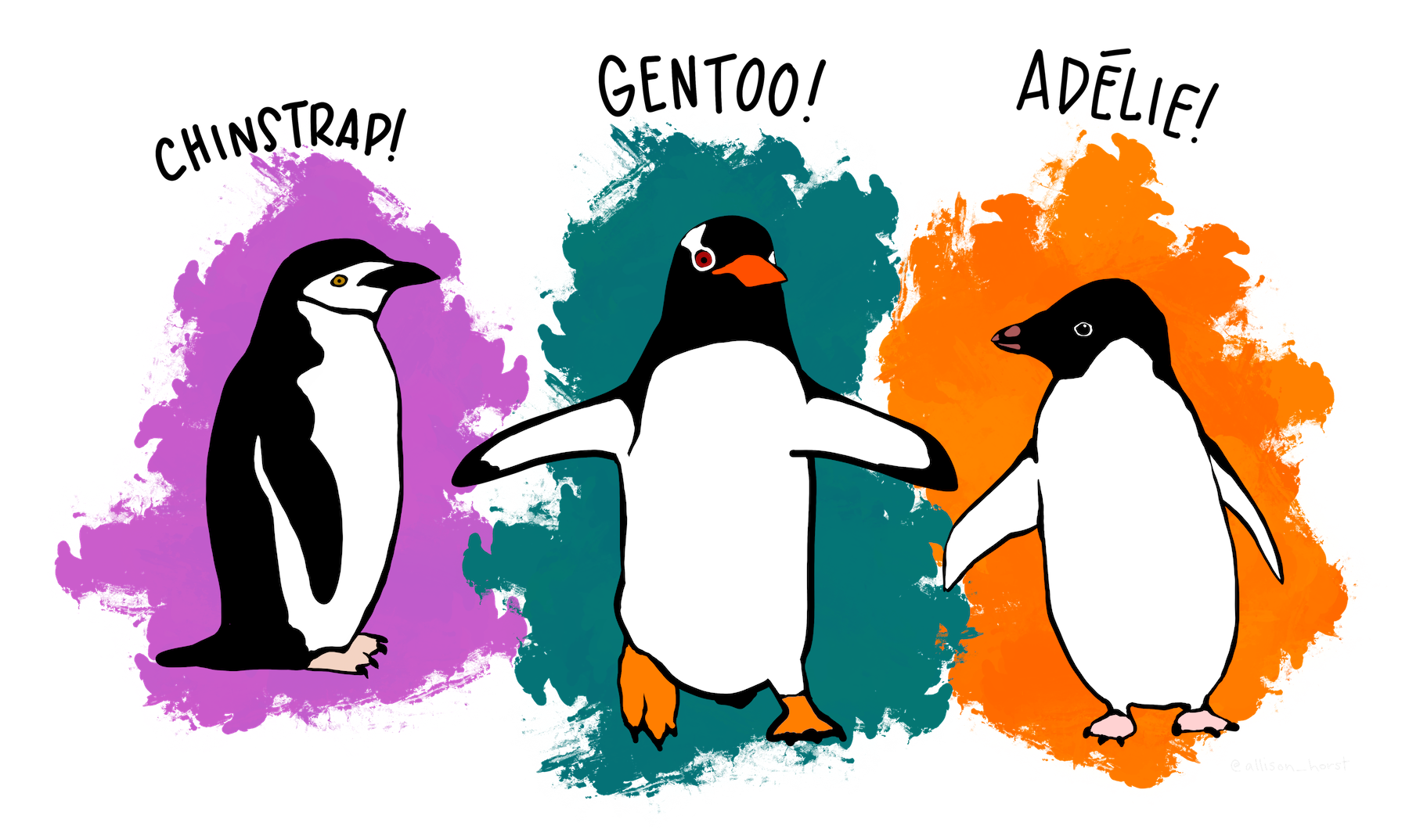
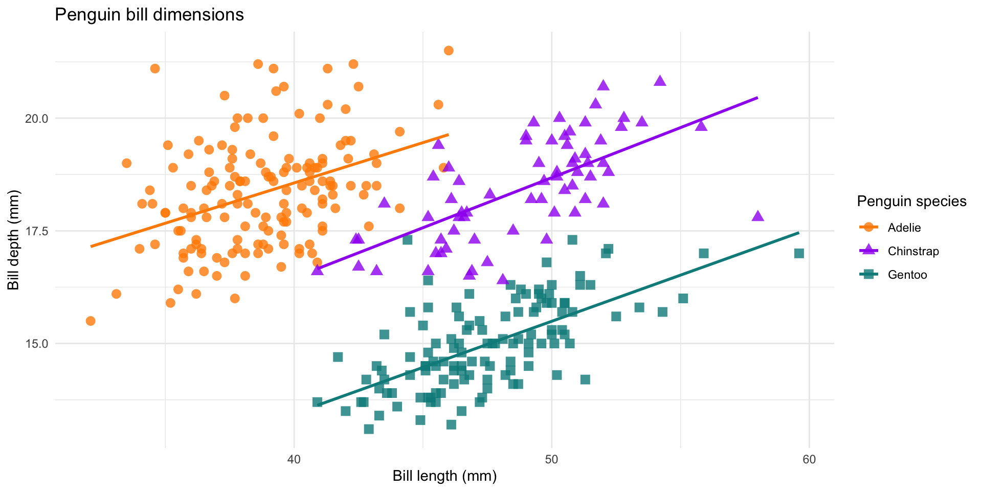
palmerpenguins is another R example data set with data on three penguin species
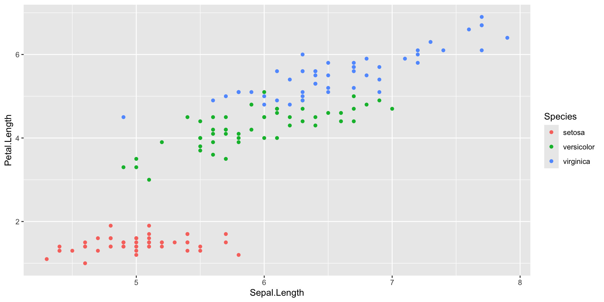
Introduction to ggplot2 package
Task 1.2
Make a similar plot
Introduction to pipes
Imagine baking a cake

Introduction to pipes
Imagine baking a cake
Introduction to pipes
Imagine baking a cake
Introduction to pipes
Imagine baking a cake
Introduction to pipes
Imagine baking a cake
Introduction to dplyr package
Useful for plotting
ggplot(data = irisS, aes(x = Species, colour = Species)) +      # Set up ggplot and columns used in all layers
  geom_point(data = iris, aes(y = Petal.Width),                 # Take raw date for point layer
             position = position_jitter()) +                    # Shuffle points along x axis
  geom_errorbar(aes(ymin = mean_petal_width - sd_petal_width,   # Take summary data for errorbars
                    ymax = mean_petal_width + sd_petal_width),
                width = 0.2) +
  geom_point(data = irisS, aes(y = mean_petal_width),           # Plot the mean on top
             shape = 21, size = 3, fill = "white") +            # with a larger point
  theme_classic()+
  theme(legend.position = "None")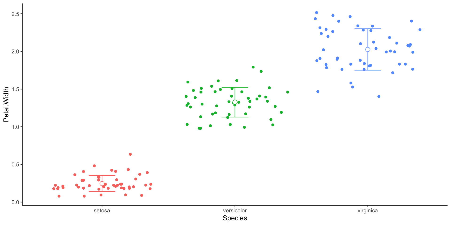
General Tips